Getting R markdown to play with jekyll
[R blog This post is an attempt to get R
Markdown to render on a
jekyll website. The prolific Yihui Xie has a github
repository yihui/blogdown to
demonstrate how to do this using blogdown and knitr. There is also some
documentation available.
Jekyll isn’t well supported by blogdown so I needed to hack a few things
together to get them to work well.
I’m going to test out a few things including making sure that plots and equations show up on the website. The code below mainly follows some example code by Jeromy Anglin that I found while learning online.
Prepare for analyses
set.seed(1234)
library(ggplot2)
Basic console output
To insert an R code chunk, you can type it manually or just press Chunks - Insert chunks or use the shortcut key. This will produce the following code chunk:
Pressing tab when inside the braces will bring up code chunk options.
The following R code chunk labelled basicconsole is as follows:
    x <- 1:10
    y <- round(rnorm(10, x, 1), 2)
    df <- data.frame(x, y)
    df
    ##     x     y
    ## 1   1 -0.21
    ## 2   2  2.28
    ## 3   3  4.08
    ## 4   4  1.65
    ## 5   5  5.43
    ## 6   6  6.51
    ## 7   7  6.43
    ## 8   8  7.45
    ## 9   9  8.44
    ## 10 10  9.11
The code chunk input and output is then displayed as follows:
x <- 1:10
y <- round(rnorm(10, x, 1), 2)
df <- data.frame(x, y)
df
## x y
## 1 1 0.52
## 2 2 1.00
## 3 3 2.22
## 4 4 4.06
## 5 5 5.96
## 6 6 5.89
## 7 7 6.49
## 8 8 7.09
## 9 9 8.16
## 10 10 12.42Plots
Images generated by knitr are saved in a figures folder. However, they also appear to be represented in the HTML output using a data URI scheme. This means that you can paste the HTML into a blog post or discussion forum and you don’t have to worry about finding a place to store the images; they’re embedded in the HTML.
Simple plot
Here is a basic plot using base graphics:
plot(x)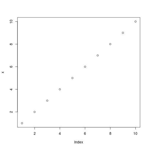
plot(x)
Note that unlike traditional Sweave, there is no need to write fig=TRUE.
ggplot2 plot
ggplot plots work well:
qplot(x, y, data=df, geom="point") + geom_line(colour="red")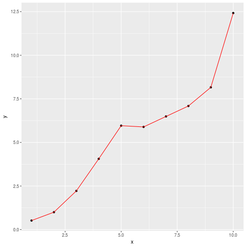
R Code chunk features
Create Markdown code from R
The following code hides the command input (i.e., echo=FALSE), and outputs the content directly as code (i.e., results=asis, which is similar to results=tex in Sweave).
Here are some dot points

* The value of y[1] is 0.52
* The value of y[2] is 1
* The value of y[3] is 2.22
Here are some dot points
- The value of y[1] is 0.52
- The value of y[2] is 1
- The value of y[3] is 2.22
Create Markdown table code from R
x | y
--- | ---
1 | 0.52
2 | 1
3 | 2.22
4 | 4.06
5 | 5.96
6 | 5.89
7 | 6.49
8 | 7.09
9 | 8.16
10 | 12.42
| x | y |
|---|---|
| 1 | 0.52 |
| 2 | 1 |
| 3 | 2.22 |
| 4 | 4.06 |
| 5 | 5.96 |
| 6 | 5.89 |
| 7 | 6.49 |
| 8 | 7.09 |
| 9 | 8.16 |
| 10 | 12.42 |
Control output display
The following code suppresses display of R input commands (i.e., echo=FALSE)
and removes any preceding text from console output (comment=""; the default is comment="##").
      x    y
    1 1 0.52
    2 2 1.00
    3 3 2.22
    4 4 4.06
    5 5 5.96
    6 6 5.89
  x    y
1 1 0.52
2 2 1.00
3 3 2.22
4 4 4.06
5 5 5.96
6 6 5.89
Test syntax highlighting
library(MASS)
MASS::fbeta
## function (x, alpha, beta)
## {
## x^(alpha - 1) * (1 - x)^(beta - 1)
## }
## <bytecode: 0x20fe768>
## <environment: namespace:MASS># testing a comment
print(paste("This is a test", "of string coloring", sep=" "))## [1] "This is a test of string coloring"a <- c(1,2,3)
b <- "red"Control figure size
The following is an example of a smaller figure using fig.width and fig.height options.
plot(x)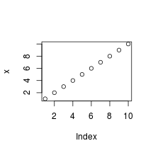
plot(x)
Basic markdown functionality
For those not familiar with standard Markdown, the following may be useful. See the source code for how to produce such points. However, RStudio does include a Markdown quick reference button that adequately covers this material.
Dot Points
Simple dot points:
- Point 1
- Point 2
- Point 3
and numeric dot points:
- Number 1
- Number 2
- Number 3
and nested dot points:
- A
- A.1
- A.2
- B
- B.1
- B.2
Equations
Equations are included by using LaTeX notation and including them either between single dollar signs (inline equations) or double dollar signs (displayed equations).
There are inline equations such as \( y_i = \alpha + \beta x_i + e_i \).
And displayed formulas:
Tables
Tables can be included using the following notation
| A | B | C |
|---|---|---|
| 1 | Male | Blue |
| 2 | Female | Pink |
Hyperlinks
- Here is a link to Wikipedia.
Images
Here’s an example image:

Code
Here is Markdown R code chunk displayed as code:
    x <- 1:10
    x
## [1] 1 2 3 4 5 6 7 8 9 10
And then there’s inline code such as x <- 1:10.
Quote
Let’s quote some stuff:
To be, or not to be, that is the question: Whether ‘tis nobler in the mind to suffer The slings and arrows of outrageous fortune,
Conclusion
- R Markdown is awesome.
- The ratio of markup to content is excellent.
- For exploratory analyses, blog posts, and the like R Markdown will be a powerful productivity booster.
- For journal articles, LaTeX will presumably still be required.
Equivalent of Sexpr
Question: Is there an R Markdown equivalent to Sexpr in Sweave?.
Answer: Include the code between brackets of “backick r space” and “backtick”. E.g., R calculates this in the source code inline 2 + 2 = 4 .