Analyzing Developmental Trajectories

A developmental trajectory describes the course of a behavior over age or time. Daniel Nagin pioneered a method called Group-based Trajectory Modeling to cluster these trajectories into groups. Link. This method is quite popular in the medical and social sciences. In this post I will take a look at his paper from 1999 - Analyzing Developmental Trajectories - A Semiparametric Group-based approach and provide some code in R to work through the datasets.

Datasets

There are two interesting datasets associated with this paper. The first is from the Cambridge study of Delinquint Development. It tracked 411 British males from a working area of London. Data collection began in the early 60s when the boys were 8 years old and continued till they were around 32. It included criminal convictions and measured variables related to a number of factors including psychological makeup, family circumstances, parenting behavior and performance in school/work.

The second dataset is a study of 1037 White males of French ancestry. This also measures similar variables to the Cambridge study.

We shall mainly focus on the Cambridge study.

Cambridge Study

library(foreign)
# read in the data
cambridge <- read.dta("https://www.andrew.cmu.edu/user/bjones/traj/data/cambrdge.dta")

This dataset has many columns and we can make some educated guesses about what is in them

• x01-x23 : Offense Counts (Number of offense counts in a year)
• x24-x46 : Unknown
• t1-t23 : Age
• tt1-tt23 : Scaled Age
• p1-p23 : Prevalence (Whether an offense was committed that year or not)
• y10 : ID
• other y’s : Unknown (Probably covariates)

We will mainly be working with the Offense Counts but first let’s convert this dataset from wide to long. The dplyr toolset makes this easy.

library(dplyr)
library(tidyr)
library(readr)

# Convert Cambridge from wide to long format
# ID, TimeIdx (1-23), Age, Offense Count, Prevalence
# We drops the covariates and only keep the time series
cambridge_long <- cambridge %>%
  rename(ID=y10) %>%
  select(-starts_with("y")) %>% # drop covariates
  select(-starts_with("tt")) %>% # drop scaled age
  select(-(x24:x46)) %>% # drop unknown x variables
  gather(variable, value, -ID) %>%
  mutate(TimeIdx = parse_number(variable)) %>%
  mutate(variable = gsub("\\d", "", x=variable)) %>%
  spread(variable, value) %>%
  select(ID, TimeIdx, Age=t, Prevalence=p, OffCount=x) 

# A sampling of rows from the dataset
cambridge_long %>% slice(c(1:3, 20:23, 100:103, 7800:7804)) %>% print()

## # A tibble: 16 x 5
##       ID TimeIdx   Age Prevalence OffCount
##    <dbl>   <dbl> <dbl>      <dbl>    <dbl>
##  1     1       1    10          0        0
##  2     1       2    11          0        0
##  3     1       3    12          0        0
##  4     1      20    29          0        0
##  5     1      21    30          0        0
##  6     1      22    31          0        0
##  7     1      23    32          0        0
##  8     5       8    17          0        0
##  9     5       9    18          0        0
## 10     5      10    19          1        1
## 11     5      11    20          1        1
## 12   347       3    12          0        0
## 13   347       4    13          1        3
## 14   347       5    14          1        2
## 15   347       6    15          0        0
## 16   347       7    16          1        2

We look at the average number of offense counts by the boys ages and put some confidence intervals around the mean.

library(ggplot2)
ggplot(cambridge_long, aes(Age, OffCount)) + 
  stat_summary(fun.y="mean", geom="line") +
  stat_summary(geom='ribbon', fun.data='mean_cl_boot', alpha=0.2) +
  labs(title="Mean Offense Count by Age", 
       y= "Mean Offense Count")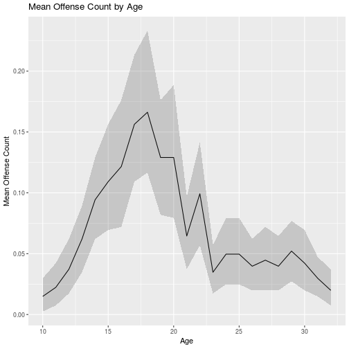

It looks like males commit a lot of offenses in the mid/late teens compared to the other years.

Fitting a Group-Based Trajectory model

library(flexmix)
set.seed(1)

num_components <- 3
ages <- 10:32

m <- flexmix(OffCount ~ Age + I(Age^2) | ID, k=num_components,
             model=FLXMRglm(family="poisson"),
             data=cambridge_long)
m

## 
## Call:
## flexmix(formula = OffCount ~ Age + I(Age^2) | ID, data = cambridge_long, 
##     k = num_components, model = FLXMRglm(family = "poisson"))
## 
## Cluster sizes:
##    1    2    3 
## 6946  644 1679 
## 
## convergence after 86 iterations

summary(m)

## 
## Call:
## flexmix(formula = OffCount ~ Age + I(Age^2) | ID, data = cambridge_long, 
##     k = num_components, model = FLXMRglm(family = "poisson"))
## 
##         prior size post>0 ratio
## Comp.1 0.7104 6946   8073 0.860
## Comp.2 0.0676  644   2323 0.277
## Comp.3 0.2220 1679   9062 0.185
## 
## 'log Lik.' -1909 (df=11)
## AIC: 3840   BIC: 3918

cambridge_long$Cluster <- clusters(m)

GetAgeClusterPred <- function(age, k)  {
  p <- parameters(m, component=k)
  exp(p[1] + p[2] * age + p[3] * age^2)
}

predictions <- expand.grid(Age=ages, Cluster=1:num_components) %>% 
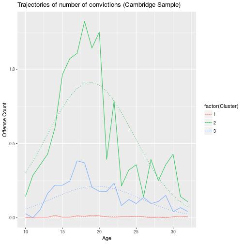
        rowwise() %>% mutate(OffCount=GetAgeClusterPred(Age, Cluster) )

ggplot(cambridge_long, aes(Age, OffCount, color=factor(Cluster))) +
  stat_summary(fun.y=mean, geom="line", alpha=0.8) + 
  geom_line(data=predictions, aes(color=factor(Cluster)), 
    linetype="dotted") +
  labs(y="Offense Count", 
    title="Trajectories of number of convictions (Cambridge Sample)")